Practical Notes for Alevels

I have compiled all the code into a single page for quick viewing of chapters

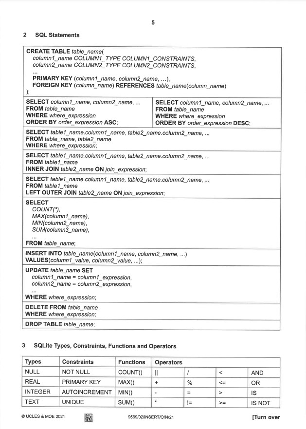
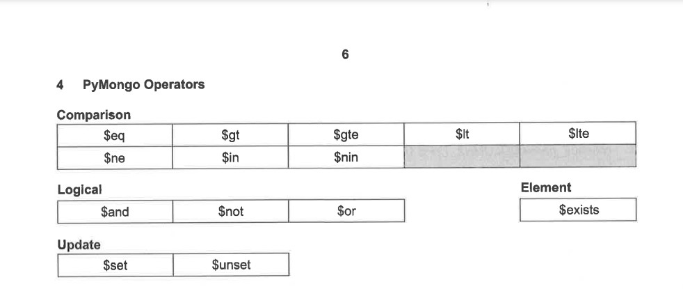
CRUD Operations on a List

Create: Use a for loop to add numbers from 1 to 10 into the list.
Read: Print the list to view its contents.
Update: Modify the value at a specific index (e.g., set the value at index 0 to 2).
Delete: Use pop() to remove the last element or pop(index) to remove an element at a specific index.

listA = []
#create items 1 - 10 in listA using for loop
for i in range(10):
    listA.append(i+1)

#read - find index of 3 in listA
print(listA)

#update - change value at an index in listA
listA[0] = 2
print(listA)

#delete - remove a value from the list
listA.pop() #deletes last value by default
print(listA)

listA.pop(0) #deletes a value at an index
print(listA)

---------------------------------------

[1, 2, 3, 4, 5, 6, 7, 8, 9, 10]
[2, 2, 3, 4, 5, 6, 7, 8, 9, 10]
[2, 2, 3, 4, 5, 6, 7, 8, 9]
[2, 3, 4, 5, 6, 7, 8, 9]

CRUD Operations on a Fixed-Size Array

In A-Levels, we do not use a real array data structure as seen in other programming contexts.
Instead, we simulate arrays using Python's list data type.
The fixed size of an array is represented by initializing a list with a specific number of None elements.
Operations like inserting, reading, updating, and deleting values can be performed on this simulated array.
This approach helps in understanding the basic functionality of arrays without relying on external libraries or native array structures.

Create: Initialize an array with a fixed size (5) filled with None.
Insert: Use a for loop to add values 1 to 5 into the array.
Read: Print the array to view its current contents.
Update: Modify the value at a specific index (e.g., set index 0 to 99).
Delete: Simulate removal by setting the last or specific index to None.

# Create an array
size = 5  # the array can only store 5 variables
arr = [None] * size

# Create items 1 - 5 in arr using a for loop
for i in range(5):
    arr[i] = i + 1

# Read - Print the array
print(arr)

# Update - Change value at index 0
arr[0] = 99
print(arr)

# Delete - Remove the last element by setting it to None
arr[-1] = None
print(arr)

# Delete - Remove the value at index 0
arr[0] = None
print(arr)

---------------------------------------

[1, 2, 3, 4, 5]
[99, 2, 3, 4, 5]
[99, 2, 3, 4, None]
[None, 2, 3, 4, None]

CRUD Operations on a Dictionary

Create

A dictionary is created with key-value pairs.
Keys include name, age, class, and subjects.

student = {'name': 'Tom', 'age': 17, 'class': '24/12', 'subjects': ['math', 'computing', 'physics', 'economics']}
print(student)

--------------------------------------- {'name': 'Tom', 'age': 17, 'class': '24/12', 'subjects': ['math', 'computing', 'physics', 'economics']}

Read

Access dictionary values using get() or direct indexing.
get() is safer as it does not throw an error for missing keys.

print(student.get('age'))  # Output: 17
print(student.get('id'))   # Output: None

---------------------------------------

17
None

Update

Update values of keys or modify nested elements (e.g., a list inside the dictionary).

student['class'] = '24/13'  # Update class
student['subjects'][1] = 'biology'  # Update subject
print(student)

--------------------------------------- {'name': 'Tom', 'age': 17, 'class': '24/13', 'subjects': ['math', 'biology', 'physics', 'economics']}

Delete

Use del or pop() to remove key-value pairs.

del student['age']
student.pop('subjects')
print(student)

--------------------------------------- {'name': 'Tom', 'class': '24/13'}

Insert

Add new key-value pairs to the dictionary.

student['teacher'] = 'Mr Tan'
print(student)

--------------------------------------- {'name': 'Tom', 'class': '24/13', 'teacher': 'Mr Tan'}

Dictionary Operations Summary

Keys: Use student.keys() to display all keys.
Values: Use student.values() to display all values.
Items: Use student.items() to get key-value pairs.
Length: Use len() to get the size of the dictionary.

print(student.keys())
print(student.values())
print(student.items())
print(len(student))

---------------------------------------

dict_keys(['name', 'class', 'teacher'])
dict_values(['Tom', '24/13', 'Mr Tan'])
dict_items([('name', 'Tom'), ('class', '24/13'), ('teacher', 'Mr Tan')])
3

String Operations

1. String Creation

Strings can be created using single, double, or triple quotes for multiline strings.

string1 = 'Hello'
string2 = "World"
string3 = '''This is
a multiline string'''
print(string1)
print(string2)
print(string3)

---------------------------------------

Hello
World
This is
a multiline string

2. Accessing Characters

Individual characters in a string can be accessed using indexing.
Negative indexing starts from the end of the string.

string = "Python"
print(string[0])  # Output: P
print(string[-1]) # Output: n

---------------------------------------

P
n

3. String Slicing

Substrings can be extracted using slicing.
Use string[start:end] to get characters from start to end (not inclusive).

string = "Python"
print(string[0:3])  # Output: Pyt
print(string[:3])   # Output: Pyt
print(string[3:])   # Output: hon

---------------------------------------

Pyt
Pyt
hon

4. String Concatenation

Combine strings using the + operator.

string1 = "Hello"
string2 = "World"
result = string1 + " " + string2
print(result)  # Output: Hello World

--------------------------------------- Hello World

5. String Multiplication

Repeat strings using the * operator.

string = "Hello"
print(string * 3)  # Output: HelloHelloHello

--------------------------------------- HelloHelloHello

6. String Length

Get the length of a string using len().

string = "Python"
print(len(string))  # Output: 6

--------------------------------------- 6

7. Using Loops

Use a for loop to iterate through each character in a string.

string = "Python"
for char in string:
    print(char)

---------------------------------------

P
y
t
h
o
n

8. Changing Case

Change the case of strings using methods like upper(), lower(), title(), etc.

string = "Python Programming"
print(string.upper())        # Output: PYTHON PROGRAMMING
print(string.lower())        # Output: python programming
print(string.title())        # Output: Python Programming
print(string.capitalize())   # Output: Python programming
print(string.swapcase())     # Output: pYTHON pROGRAMMING

---------------------------------------

PYTHON PROGRAMMING
python programming
Python Programming
Python programming
pYTHON pROGRAMMING

9. Stripping Whitespace

Remove leading, trailing, or both whitespace using strip(), lstrip(), and rstrip().

string = "  Hello World  "
print(string.strip())  # Output: Hello World

#Optional
print(string.lstrip()) # Output: Hello World  
print(string.rstrip()) # Output:   Hello World

---------------------------------------

Hello World
Hello World  
  Hello World

10. Splitting and Joining Strings

Use split() to break a string into parts.
Use join() to combine a list of strings into a single string.

string = "Python,Java,C++"
print(string.split(","))  # Output: ['Python', 'Java', 'C++']

words = ["Python", "is", "fun"]
print(" ".join(words))  # Output: Python is fun

---------------------------------------


['Python', 'Java', 'C++']
Python is fun

11. Replacing Substrings

Use replace() to replace parts of a string with another string.

string = "I like Java"
print(string.replace("Java", "Python"))  # Output: I like Python

--------------------------------------- I like Python

12. Finding Substrings

Find the position of a substring using find(). Returns -1 if not found.

string = "Python Programming"
print(string.find("Programming"))  # Output: 7
print(string.find("Java"))         # Output: -1

---------------------------------------

7
-1

13. String Formatting

Format strings using f-strings or the format() method.

name = "Alice"
age = 25
print(f"My name is {name} and I am {age} years old.")  
print("My name is {} and I am {} years old.".format(name, age))

---------------------------------------

My name is Alice and I am 25 years old.
My name is Alice and I am 25 years old.

14. String Validation

Check properties of strings using methods like isalpha(), isdigit(), isalnum(), etc.

string = "Python123"
print(string.isalpha())  # Output: False
print(string.isdigit())  # Output: False
print(string.isalnum())  # Output: True

---------------------------------------

False
False
True

15. Reversing a String

Reverse a string using slicing [::-1].

string = "Python"
print(string[::-1])  # Output: nohtyP

--------------------------------------- nohtyP

Recursive vs Iterative Approaches

1. What is Recursion?

Recursion is a method where a function calls itself to solve a problem. It breaks the problem into smaller sub-problems until reaching a base case.

Advantages:
- Simplifies code for problems that have a recursive structure (e.g., factorial, Fibonacci, tree traversal).
Disadvantages:
- Consumes more memory due to recursive function calls.
- Risk of stack overflow for deep recursion.

2. What is Iteration?

Iteration uses loops (e.g., for, while) to repeatedly execute a block of code until a condition is met.

Advantages:
- Consumes less memory compared to recursion.
- No stack overflow risk.
Disadvantages:
- Can be harder to implement for problems with recursive structures.

3. Comparison: Factorial Calculation

Recursive Implementation

def factorial_recursive(n):
    if n == 0 or n == 1:
        return 1  # Base case
    else:
        return n * factorial_recursive(n - 1)  # Recursive case

# main
print(factorial_recursive(5))  # Output: 120

--------------------------------------- 120

Iterative Implementation

def factorial_iterative(n):
    result = 1
    for i in range(1, n + 1):
        result *= i
    return result

# main
print(factorial_iterative(5))  # Output: 120

--------------------------------------- 120

4. Comparison: Fibonacci Calculation

Recursive Implementation

def fibonacci_recursive(n):
    if n == 0:
        return 0
    elif n == 1:
        return 1
    else:
        return fibonacci_recursive(n - 1) + fibonacci_recursive(n - 2)

# main
print(fibonacci_recursive(6))  # Output: 8

--------------------------------------- 8

Iterative Implementation

def fibonacci_iterative(n):
    if n == 0:
        return 0
    elif n == 1:
        return 1
    a, b = 0, 1
    for _ in range(2, n + 1):
        a, b = b, a + b
    return b

# main
print(fibonacci_iterative(6))  # Output: 8

--------------------------------------- 8

5. Key Differences

Aspect	Recursion	Iteration
Definition	A function calls itself.	Repeated execution using loops.
Memory Usage	Higher due to recursive calls and stack frames.	Lower as no additional stack is used.
Performance	Can be slower due to overhead of function calls.	Faster as no function call overhead.
Suitability	Best for problems with recursive structures.	Best for iterative tasks.

File I/O Operations

1. Reading from a Text File

Open a .txt file in read mode using open('filename', 'r').
Use readlines() to read all lines into a list.
Iterate through the list to process each line.

with open('filename.txt', 'r') as infile:
    lines = infile.readlines()
    for line in lines:
        print(line)

2. Reading from a CSV File

Open a .csv file in read mode using open('filename', 'r').
Use the csv.reader() module to read rows as lists.
Use next() to skip the header row if present.

import csv

with open('filename.csv', 'r') as infile:
    lines = csv.reader(infile)
    next(lines)  # Skip the header row
    for line in lines:
        print(line)

3. Reading from a JSON File

Open a .json file in read mode using open('filename', 'r').
Use json.load() to parse the JSON file into a Python dictionary or list.

import json

with open('filename.json', 'r') as infile:
    data = json.load(infile)
    for item in data:
        print(item)

4. Reading Text File Data

Use slicing to read specific fields from each line in a text file.
For example, read student_id, name, and class_id based on their positions in the line.

people.txt

1.  01John Doe           24/12
2.  02Jane Smith         25/13

with open('people.txt', 'r') as infile:
    lines = infile.readlines()
    print(lines)
    for line in lines:
        student_id = line[0:2]
        name = line[2:22]
        classid = line[22:].strip()
        print(student_id)
        print(name)
        print(classid)

---------------------------------------

01
John Doe           
24/12
02
Jane Smith         
25/13

5. Writing to a Text File

Open a file in write mode using open('filename', 'w').
Use write() to add formatted data to the file.
Format the output using f-strings or other string formatting methods.

with open('result.txt', 'w') as outfile:
    student_id = "03"
    name = 'Ali'
    classid = '24/12'
    outfile.write(f'{student_id}{name:20}{classid}\n')

result.txt

1.  03Ali                 24/12

6. Appending to a Text File

Open a file in append mode using open('filename', 'a').
Use append() to add formatted data to a new line at the end of the file.
Format the output using f-strings or other string formatting methods.

with open('result.txt', 'a') as outfile:
    student_id = "04"
    name = 'Jack'
    classid = '25/12'
    outfile.write(f'{student_id}{name:20}{classid}\n')

result.txt

1.  03Ali                 24/12
2.  04Jack                25/12

Iterative Number Base Conversions

1. Decimal to Binary

Definition: Convert a decimal number to binary by repeatedly dividing by 2 and storing the remainders in reverse order.
Steps:
- Divide the decimal number by 2.
- Store the remainder as a binary digit.
- Repeat until the quotient is 0.
- Read the remainders in reverse order.

def decimal_to_binary(dec_num):
    bin_num = ''
    while dec_num > 0:
        remainder = dec_num % 2
        bin_num = str(remainder) + bin_num
        dec_num = dec_num // 2
    return bin_num

# main
print(decimal_to_binary(1114))  # Output: 10001011010

--------------------------------------- 10001011010

2. Decimal to Hexadecimal

Definition: Convert a decimal number to hexadecimal by repeatedly dividing by 16 and storing the remainders in reverse order.
Steps:
- Divide the decimal number by 16.
- Map the remainder to its hexadecimal equivalent.
- Repeat until the quotient is 0.
- Read the remainders in reverse order.

def decimal_to_hexadecimal(dec_num):
    dec_hex_map = {1:'1', 2:'2', 3:'3', 4:'4', 5:'5', 6:'6', 7:'7', 8:'8', 9:'9', \
    10:'A', 11:'B', 12:'C', 13:'D', 14:'E', 15:'F'}
    hex_num = ''
    while dec_num > 0:
        remainder = dec_num % 16
        hex_num = str(dec_hex_map[remainder]) + hex_num
        dec_num = dec_num // 16
    return hex_num

# main
print(decimal_to_hexadecimal(1114))  # Output: 45A

--------------------------------------- 45A

3. Decimal to Base n, where n is an integer

Definition: Convert a decimal number to base n by repeatedly dividing by n and storing the remainders in reverse order.
Steps:
- If the base is less than 10.
- Divide the decimal number by n.
- Store the remainder as a base n digit.
- Repeat until the quotient is 0.
- Read the remainders in reverse order.
- If the base is more than 10.
- You would need a hex_map similar to decimal to hexadecimal
- Do read the question for more information

def decimal_to_base(dec_num, n):
    num = ''
    while dec_num > 0:
        remainder = dec_num % n
        num = str(remainder) + num
        dec_num = dec_num // n
    return num

# main
print(decimal_to_base(1114, 8))  # Output: 2132

--------------------------------------- 2132

4. Binary to Decimal

Definition: Convert a binary number to decimal by summing the products of binary digits and positional powers of 2.

def binary_to_decimal(bin_num):
    dec_num = 0
    for i in range(len(bin_num)):
        digit = bin_num[len(bin_num) - 1 - i]
        dec_num += int(digit) * (2 ** i)
    return dec_num

# main
print(binary_to_decimal('10001011010'))  # Output: 1114

--------------------------------------- 1114

5. Hexadecimal to Decimal

Definition: Convert a hexadecimal number to decimal by summing the products of hexadecimal digits and positional powers of 16.

def hexadecimal_to_decimal(hex_num):
    hex_dec_map = {'1':1, '2':2, '3':3, '4':4, '5':5, '6':6, '7':7, '8':8, '9':9, \
    'A':10, 'B':11, 'C':12, 'D':13, 'E':14, 'F':15}
    dec_num = 0
    for i in range(len(hex_num)):
        digit = hex_num[len(hex_num) - 1 - i]
        dec_num += int(hex_dec_map[digit]) * (16 ** i)
    return dec_num

# main
print(hexadecimal_to_decimal('45A'))  # Output: 1114

--------------------------------------- 1114

You only need these 5 as you can use it to convert from one base to denary to another base. For example: binary to decimal to hexadecimal

6. Binary to Hexadecimal (OPTIONAL)

Definition: Group binary digits into groups of 4 from right to left and map directly to hexadecimal.

def binary_to_hexadecimal(bin_num):
    bin_hex_map = {'0000': '0', '0001': '1', '0010': '2', '0011': '3', \
    '0100': '4', '0101': '5', '0110': '6', '0111': '7', \
    '1000': '8', '1001': '9', '1010': 'A', '1011': 'B', \
    '1100': 'C', '1101': 'D', '1110': 'E', '1111': 'F'}
    bin_num = bin_num.zfill((len(bin_num) + 3) // 4 * 4)
    hex_num = ''
    for i in range(0, len(bin_num), 4):
        hex_num += bin_hex_map[bin_num[i:i+4]]
    return hex_num

# main
print(binary_to_hexadecimal('10001011010'))  # Output: 45A

--------------------------------------- 45A

7. Hexadecimal to Binary (OPTIONAL)

Definition: Map each hexadecimal digit directly to its 4-bit binary equivalent.

def hexadecimal_to_binary(hex_num):
    hex_bin_map = {'0': '0000', '1': '0001', '2': '0010', '3': '0011', \
    '4': '0100', '5': '0101', '6': '0110', '7': '0111', \
    '8': '1000', '9': '1001', 'A': '1010', 'B': '1011', \
    'C': '1100', 'D': '1101', 'E': '1110', 'F': '1111'}
    bin_num = ''.join(hex_bin_map[digit.upper()] for digit in hex_num)
    return bin_num

# main
print(hexadecimal_to_binary('45A'))  # Output: 10001011010

--------------------------------------- 10001011010

Recursive Number Base Conversions

1. Decimal to Binary (Recursive)

def decimal_to_binary_recursive(dec_num):
    if dec_num == 0:
        return ''
    else:
        return decimal_to_binary_recursive(dec_num // 2) + str(dec_num % 2)

# main
print(decimal_to_binary_recursive(1114))  # Output: 10001011010

--------------------------------------- 10001011010

2. Decimal to Hexadecimal (Recursive)

dec_hex_map = {1:'1', 2:'2', 3:'3', 4:'4', 5:'5', 6:'6', 7:'7', 8:'8', 9:'9', \
10:'A', 11:'B', 12:'C', 13:'D', 14:'E', 15:'F'}

def decimal_to_hexadecimal_recursive(dec_num):
    if dec_num == 0:
        return ''
    else:
        remainder = dec_num % 16
        return decimal_to_hexadecimal_recursive(dec_num // 16) + str(dec_hex_map[remainder])

# main
print(decimal_to_hexadecimal_recursive(1114))  # Output: 45A

--------------------------------------- 45A

3. Binary to Decimal (Recursive)

def binary_to_decimal_recursive(bin_num):
    if len(bin_num) == 0:
        return 0
    else:
        digit = bin_num[0]
        return int(digit) * (2 ** (len(bin_num) - 1)) + binary_to_decimal_recursive(bin_num[1:])

# main
print(binary_to_decimal_recursive('10001011010'))  # Output: 1114

--------------------------------------- 1114

4. Hexadecimal to Decimal (Recursive)

hex_dec_map = {'1':1, '2':2, '3':3, '4':4, '5':5, '6':6, '7':7, '8':8, '9':9, \
'A':10, 'B':11, 'C':12, 'D':13, 'E':14, 'F':15}

def hexadecimal_to_decimal_recursive(hex_num):
    if len(hex_num) == 0:
        return 0
    else:
        digit = hex_num[0]
        return int(hex_dec_map[digit]) * (16 ** (len(hex_num) - 1)) + hexadecimal_to_decimal_recursive(hex_num[1:])

# main
print(hexadecimal_to_decimal_recursive('45A'))  # Output: 1114

--------------------------------------- 1114

5. Binary to Hexadecimal (Recursive)

bin_hex_map = {'0000': '0', '0001': '1', '0010': '2', '0011': '3', \
'0100': '4', '0101': '5', '0110': '6', '0111': '7', \
'1000': '8', '1001': '9', '1010': 'A', '1011': 'B', \
'1100': 'C', '1101': 'D', '1110': 'E', '1111': 'F'}

def binary_to_hexadecimal_recursive(bin_num):
    padding = len(bin_num) % 4
    if padding != 0:
        bin_num = '0' * (4 - padding) + bin_num

    if len(bin_num) == 0:
        return ''
    else:
        group = bin_num[-4:]
        return binary_to_hexadecimal_recursive(bin_num[:-4]) + bin_hex_map[group]

# main
print(binary_to_hexadecimal_recursive('10001011010'))  # Output: 45A

--------------------------------------- 45A

6. Hexadecimal to Binary (Recursive)

hex_to_bin_map = {'0': '0000', '1': '0001', '2': '0010', '3': '0011', \
'4': '0100', '5': '0101', '6': '0110', '7': '0111', \
'8': '1000', '9': '1001', 'A': '1010', 'B': '1011', \
'C': '1100', 'D': '1101', 'E': '1110', 'F': '1111'}

def hexadecimal_to_binary_recursive(hex_num):
    if len(hex_num) == 0:
        return ''
    else:
        return hex_to_bin_map[hex_num[0].upper()] + hexadecimal_to_binary_recursive(hex_num[1:])

# main
print(hexadecimal_to_binary_recursive('45A'))  # Output: 10001011010

--------------------------------------- 10001011010

Data Validation Techniques

1. Presence Check

Ensures that required fields are not left empty.
Commonly used in forms where specific fields must be filled out.

data = input("Enter your name: ")
if data.strip() == "":
    print("Error: This field cannot be empty.")
else:
    print("Valid input!")

2. Length Check

Ensures that the input meets a specified length requirement (minimum or maximum).

data = input("Enter a password (min 8 characters): ")
if len(data) < 8:
    print("Error: Password must be at least 8 characters long.")
else:
    print("Valid password!")

3. Data Type Check

Validates that the input matches the expected data type (e.g., integer, float, string).

data = input("Enter a number: ")
if data.isdigit():
    print("Valid input!")
else:
    print("Error: Input must be a number.")

4. Format Check

Ensures that the input follows a specific format (e.g., email address, phone number).

data = input("Enter an email address: ")
symbol_count = 0
for char in data:
  if char = '@':
    symbol_count += 1

if count = 1:
    print("Valid email!")
else:
    print("Error: Invalid email format.")
    print("Error: Invalid email format.")

5. Range Check

Ensures that numerical input falls within a specified range.

data = int(input("Enter a number between 1 and 100: "))
if 1 <= data <= 100:
    print("Valid input!")
else:
    print("Error: Number out of range.")

6. Existence Check

Verifies that the input exists in a predefined list or database.

valid_users = ["Alice", "Bob", "Charlie"]
data = input("Enter your username: ")
if data in valid_users:
    print("Valid username!")
else:
    print("Error: Username does not exist.")

7. Check Digit

Validates numerical identifiers (e.g., ISBN, credit card numbers) using algorithms.
The calculation of the check digit depends on the question.
The given code is just an example, that you do not have to memorise.

# Example: Simple Mod-10 Check
data = "12345678"
check_digit = int(data[-1])
calculated_digit = sum(int(digit) for digit in data[:-1]) % 10
if check_digit == calculated_digit:
    print("Valid check digit!")
else:
    print("Error: Invalid check digit.")

Search Algorithms

1. Linear Search

Definition: A simple search that scans each element in a list sequentially.
Time Complexity: O(n).
Steps:
- Iterate through the list.
- Compare each element with the target value.
- If found, return the index; otherwise, return "not found".

def linear_search(A, target):
    for i in range(len(A)):
        if A[i] == target: # found
            return i
    return "not found" # not found

# main
data = [6, 2, 5, 1, 7, 10, 9, 3]
print(linear_search(data, 1)) # success
print(linear_search(data, 4)) # failure

---------------------------------------

3
"not found"

2. Binary Search

Definition: An efficient search for sorted lists by repeatedly dividing the search interval in half.
Time Complexity: O(log n).

Iterative Binary Search

def binary_search(A, target):
    low = 0
    high = len(A) - 1
    while low <= high:
        mid = (low + high) // 2
        if A[mid] == target: # found
            return mid
        elif A[mid] > target: # left half
            high = mid - 1
        else: # right half
            low = mid + 1
    return "not found"

# main
data = [1, 2, 3, 5, 6, 7, 9, 10]
print(binary_search(data, 7)) # success
print(binary_search(data, 8)) # failure

---------------------------------------

5
"not found"

Recursive Binary Search

def binary_searchr(A, target, low, high):
    if low > high:
        return -1 # not found
    mid = (low + high) // 2
    if A[mid] == target:
        return mid
    elif target < A[mid]:
        return binary_searchr(A, target, low, mid - 1) # left half
    else:
        return binary_searchr(A, target, mid + 1, high) # right half

# main
data = [6, 8, 12, 17, 19]
print(binary_searchr(data, 17, 0, len(data)-1)) # success
print(binary_searchr(data, 13, 0, len(data)-1)) # failure

---------------------------------------

3
-1

Sort Algorithms

1. Bubble Sort

Definition: A sorting algorithm that repeatedly swaps adjacent elements if they are in the wrong order.
Time Complexity: O(n²).

Non-Optimized Bubble Sort

def bubble_sort(A):
    n = len(A)
    for i in range(n):
        for j in range(n-1):
            if A[j] > A[j+1]:
                A[j], A[j+1] = A[j+1], A[j]
    return A

# main
data = [4, 7, 1, 5, 2, 8, 3, 6]
print(bubble_sort(data))

--------------------------------------- [1, 2, 3, 4, 5, 6, 7, 8]

Optimized Bubble Sort

def bubble_sort(A):
    n = len(A)
    for i in range(n):
        swapped = False
        for j in range(n-1):
            if A[j] > A[j+1]:
                A[j], A[j+1] = A[j+1], A[j]
                swapped = True
        if not swapped: # no swaps -> already sorted
            break
    return A

# main
data = [4, 7, 1, 5, 2, 8, 3, 6]
print(bubble_sort(data))

--------------------------------------- [1, 2, 3, 4, 5, 6, 7, 8]

2. Insertion Sort

Definition: A sorting algorithm that builds the sorted list one element at a time by inserting elements into their correct positions.
Time Complexity: O(n²).

Insertion Sort With key

def insertion_sort(A):
    for i in range(1, len(A)):
        key = A[i]
        j = i - 1
        while j >= 0 and key < A[j]:
            A[j+1] = A[j]
            j -= 1
        A[j+1] = key
    return A

# main
data = [4, 7, 1, 5, 2, 8, 3, 6]
print(insertion_sort(data))

--------------------------------------- [1, 2, 3, 4, 5, 6, 7, 8]

Alternative Insertion Sort

def insertion_sort(A):
    for i in range(1, len(A)):
      j = i
      while A[j-1] > A[j] and j > 0:
        A[j-1], A[j] = A[j], A[j-1]
        j -= 1
    return A  

# main
data = [4, 7, 1, 5, 2, 8, 3, 6]
print(insertion_sort(data))

--------------------------------------- [1, 2, 3, 4, 5, 6, 7, 8]

3. Quick Sort

Definition: A divide-and-conquer algorithm that selects a pivot and partitions the list into smaller and larger elements, then recursively sorts the sublists.
Time Complexity: O(n log n) on average.

With List Comprehension

def quicksort(A):
    if len(A) <= 1:
        return A
    pivot = A[len(A) // 2]
    left = [x for x in A if x < pivot]
    middle = [x for x in A if x == pivot]
    right = [x for x in A if x > pivot]
    return quicksort(left) + middle + quicksort(right)

# main
data = [4, 7, 1, 5, 2, 8, 3]
print(quicksort(data))

--------------------------------------- [1, 2, 3, 4, 5, 6, 7, 8]

Without List Comprehension

def quicksort(A):
    if len(A) <= 1: # terminating cases (0 or 1 item)
        return A

    pivot = A[len(A) // 2] # midpoint
    left = []
    middle = []
    right = []

    for element in A:
        if element < pivot:
            left.append(element)
        elif element == pivot:
            middle.append(element)
        else:
            right.append(element)

    return quicksort(left) + middle + quicksort(right) # recursive cases

# main
data = [4, 7, 1, 5, 2, 8, 3]
print(quicksort(data))

--------------------------------------- [1, 2, 3, 4, 5, 6, 7, 8]

Without List Comprehension Simplified

def quicksort(A):
    if len(A) <= 1: # terminating cases (0 or 1 item)
        return A

    pivot = A[len(A) // 2] # midpoint
    left = [] # items less than pivot
    right = [] # items more than pivot

    for element in A:
        if element < pivot:
            left.append(element)
        elif element > pivot:
            right.append(element)

    return quicksort(left) + [pivot] + quicksort(right) # recursive cases

# main
data = [4, 7, 1, 5, 2, 8, 3]
print(quicksort(data))

--------------------------------------- [1, 2, 3, 4, 5, 6, 7, 8]

4. Merge Sort

Definition: A divide-and-conquer algorithm that splits the list into halves, sorts each half, and merges them.
Time Complexity: O(n log n).

Iterative Merge Sort

def merge_sorti(A):
    n = len(A)
    if n <= 1:
    return A

    left = merge_sorti(A[:n//2])
    right = merge_sorti(A[n//2:])

    i = j = k = 0
    sorted_list = [None] * n

    while i < len(left) and j < len(right):
    if left[i] < right[j]:
        sorted_list[k] = left[i]
        i += 1
    else:
        sorted_list[k] = right[j]
        j += 1
    k += 1

    while i < len(left):
    sorted_list[k] = left[i]
    i += 1
    k += 1

    while j < len(right):
    sorted_list[k] = right[j]
    j += 1
    k += 1

    return sorted_list

# main
data = [4, 7, 1, 5, 2, 8, 3, 6]
print(merge_sorti(data))

--------------------------------------- [1, 2, 3, 4, 5, 6, 7, 8]

Recursive Merge Sort

def merge_sortr(A):
    if len(A) <= 1:
        return A
    mid = len(A) // 2
    left = merge_sortr(A[:mid])
    right = merge_sortr(A[mid:])
    return merge(left, right)

def merge(left, right):
    merged_list = []
    i = j = 0
    while i < len(left) and j < len(right):
        if left[i] < right[j]:
            merged_list.append(left[i])
            i += 1
        else:
            merged_list.append(right[j])
            j += 1
    merged_list += left[i:]
    merged_list += right[j:]
    return merged_list

# main
data = [4, 7, 1, 5, 2, 8, 3, 6]
print(merge_sortr(data))

--------------------------------------- [1, 2, 3, 4, 5, 6, 7, 8]

Object-Oriented Programming (OOP)

Object-Oriented Programming is a paradigm that uses objects and classes to structure and organize code. Below are the fundamental concepts of OOP with examples:

1. Class and Object

Class: A blueprint for creating objects.
Object: An instance of a class, with its own data and behavior.

class Car:
    def __init__(self, brand, speed):
        self.brand = brand
        self.speed = speed

    def drive(self):
        return f"{self.brand} is driving at {self.speed} km/h."

# Main
car1 = Car("Toyota", 120)
print(car1.drive())

--------------------------------------- Toyota is driving at 120 km/h.

2. Encapsulation

Encapsulation bundles data and methods together, restricting access using private attributes.

class BankAccount:
    def __init__(self, balance):
        self.__balance = balance  # Private attribute

    def deposit(self, amount):
        self.__balance += amount

    def get_balance(self):
        return self.__balance

# Main
account = BankAccount(1000)
account.deposit(500)
print(account.get_balance())

--------------------------------------- 1500

3. Inheritance

Inheritance enables a class (child) to reuse the properties and methods of another class (parent).

class Animal:
    def __init__(self, name):
        self.name = name

    def speak(self):
        return f"{self.name} makes a sound."

class Dog(Animal):
    def speak(self):
        return f"{self.name} barks."

# Main
dog = Dog("Buddy")
print(dog.speak())

--------------------------------------- Buddy barks.

4. Polymorphism

Polymorphism allows methods in different classes to have the same name but different behaviors.

class Bird:
    def fly(self):
        return "Birds can fly."

class Penguin(Bird):
    def fly(self):
        return "Penguins cannot fly."

# Main
animals = [Bird(), Penguin()]
for animal in animals:
    print(animal.fly())

---------------------------------------

Birds can fly.
Penguins cannot fly.

Linked List

A linked list is a linear data structure in which elements (nodes) are connected using pointers.

Always read the question as they can often hint or guide you on what you have to do.
Questions may also ask you to come up with new functions.
Hence it is crucial to understand how the code works and be able to adapt and modify it.

Below are key operations and examples:

1. Structure of a Node

A Node contains two parts:
- Data: Stores the actual data of the node.
- Pointer: Stores the reference to the next node.

class Node:
    def __init__(self, data, pointer=None):
        self.__data = data
        self.__pointer = pointer

    def getPointer(self):
        return self.__pointer

    def setPointer(self, pointer):
        self.__pointer = pointer

    def getData(self):
        return self.__data

    def setData(self, data):
        self.__data = data

2. Operations in a Linked List

The LinkedList class provides methods to manipulate and traverse the list.
Below are examples of operations like inserting, deleting, and displaying elements.

a) Inserting at the Head

Adds a new node at the beginning of the list.

class LinkedList:
    def insertHead(self, data):
        newnode = Node(data)
        if self.isEmpty():
            self.__head = newnode
        else:
            newnode.setPointer(self.__head)
            self.__head = newnode

b) Inserting at the Tail

Adds a new node at the end of the list.

def insertTail(self, data):
    newnode = Node(data)
    if self.isEmpty():
        self.__head = newnode
    else:
        curr = self.__head
        while curr.getPointer() != None:
            curr = curr.getPointer()
        curr.setPointer(newnode)

c) Deleting the Head

Removes the first node in the list.

def deleteHead(self):
    if self.isEmpty():
        print(f'Nothing to delete')
    else:
        self.__head = self.__head.getPointer()

d) Calculating the Length

Counts the number of nodes in the list.

def length(self):
    count = 0
    curr = self.__head
    while curr != None:
        count += 1
        curr = curr.getPointer()
    return count

e) Displaying the List

Traverses and prints all nodes in the list.

def display(self):
    if self.isEmpty():
        print(f'List is Empty')
    else:
        curr = self.__head
        while curr != None:
            print(f'{curr.getData()}')
            curr = curr.getPointer()

3. Example Usage

Below is an example demonstrating how to use the LinkedList class:

# Main
linked_list = LinkedList()

# Insert nodes
linked_list.insertHead(10)
linked_list.insertTail(20)
linked_list.insertTail(30)

# Display list
linked_list.display()

# Delete head
linked_list.deleteHead()
linked_list.display()

# Length of list
print(f'Length: {linked_list.length()}')

---------------------------------------

10
20
30
20
30
Length: 2

Stack and Queue

Stacks and Queues are fundamental data structures. They are used for managing collections of data with specific rules:

Stack (LIFO): Last-In, First-Out order.
Queue (FIFO): First-In, First-Out order.

1. Stack

A stack is a linear data structure that follows the LIFO principle.
Push: Add an element to the top of the stack.
Pop: Remove the top element.
Peek: View the top element without removing it.

a) Example Using Python Built-in List

x = []
x.append(2)  # First In
x.append(5)
x.append(1)
x.append(3)
x.append(9)
print(x)  # Output: [2, 5, 1, 3, 9]
x.pop()   # Last Out
print(x)  # Output: [2, 5, 1, 3]

b) Implementing Stack Class

class Stack:
    def __init__(self):
        self.items = []

    def is_empty(self):
        return len(self.items) == 0

    def push(self, item):
        self.items.append(item)

    def pop(self):
        if not self.is_empty():
            return self.items.pop()
        else:
            raise IndexError("pop from empty stack")

    def peek(self):
        if not self.is_empty():
            return self.items[-1]
        else:
            raise IndexError("peek from empty stack")

    def size(self):
        return len(self.items)

# Stack example
stack = Stack()
stack.push(1)
stack.push(2)
stack.push(3)
print(stack.pop())  # Output: 3
print(f'Value of last element: {stack.peek()}')  # Output: 2
print(f'Size of stack: {stack.size()}')  # Output: 2

---------------------------------------

3
Value of last element: 2
Size of stack: 2

2. Queue

A queue is a linear data structure that follows the FIFO principle.
Enqueue: Add an element to the end of the queue.
Dequeue: Remove the front element.
Front: View the front element without removing it.

a) Example Using Python Built-in List

x = []
x.append(2)  # First In
x.append(5)
x.append(1)
x.append(3)
x.append(9)
print(x)  # Output: [2, 5, 1, 3, 9]
x.pop(0)  # First Out
print(x)  # Output: [5, 1, 3, 9]

b) Implementing Queue Class

class Queue:
    def __init__(self):
        self.items = []

    def is_empty(self):
        return len(self.items) == 0

    def enqueue(self, item):
        self.items.append(item)

    def dequeue(self):
        if not self.is_empty():
            return self.items.pop(0)
        else:
            raise IndexError("dequeue from empty queue")

    def front(self):
        if not self.is_empty():
            return self.items[0]
        else:
            raise IndexError("front from empty queue")

    def size(self):
        return len(self.items)

# Queue example
queue = Queue()
queue.enqueue('a')
queue.enqueue('b')
queue.enqueue('c')
print(queue.dequeue())  # Output: 'a'
print(f'Value of first element: {queue.front()}')  # Output: 'b'
print(f'Size of queue: {queue.size()}')  # Output: 2

---------------------------------------

'a'
Value of first element: b
Size of queue: 2

Binary Search Tree (BST) Implementations

1. Iterative BST Implementation

Node Class:
- Represents a single node in the tree with data, left, and right pointers.
Insertion:
- If the tree is empty, the node becomes the root.
- Traverse the tree iteratively:
  - Move left if the value is smaller than the current node.
  - Move right if the value is larger.
  - Insert the value when a None position is found.
Search:
- Traverse the tree iteratively:
  - If the value matches the current node, return True.
  - Move left or right based on comparisons.
  - Return False if the value isn’t found before reaching a leaf.
Traversals:
- Inorder: Left → Root → Right.
- Preorder: Root → Left → Right.
- Postorder: Left → Right → Root.
- Reverse: Right → Left → Root.
Maximum/Minimum:
- For maximum, move right until the last node.
- For minimum, move left until the last node.

class Node:
def __init__(self, data):
    self.data = data
    self.left = None
    self.right = None

class BST:
    def __init__(self):
        self.root = None

    def insert(self, data):
        node = Node(data)
        if self.root is None:
            self.root = node
            return
        else:
            cur = self.root
            while cur:
                if cur.data > data:
                    if cur.left is None:
                        cur.left = node
                        return
                    else:
                        cur = cur.left
                else:
                    if cur.right is None:
                        cur.right = node
                        return
                    else:
                        cur = cur.right

    def search(self, data):
        if self.root is None:
            return 'empty bst'
        else:
            cur = self.root
            while cur:
                if cur.data == data:
                    return True
                elif cur.data > data:
                    if cur.left is None:
                        return False
                    else:
                        cur = cur.left
                else:
                    if cur.right is None:
                        return False
                    else:
                        cur = cur.right

    def inorder(self):
        def helper(node):
            if node:
                helper(node.left)
                print(node.data, end=' ')
                helper(node.right)
        helper(self.root)
        print()

    def preorder(self):
        def helper(node):
            if node:
                print(node.data, end=' ')
                helper(node.left)
                helper(node.right)
        helper(self.root)
        print()

    def postorder(self):
        def helper(node):
            if node:
                helper(node.left)
                helper(node.right)
                print(node.data, end=' ')
        helper(self.root)
        print()

    def reverse(self):
        def helper(node):
            if node:
                helper(node.right)
                helper(node.left)
                print(node.data, end=' ')
        helper(self.root)
        print()

    def maximum(self):
        cur = self.root
        while cur:
            if cur.right is None:
                return cur.data
            else:
                cur = cur.right

    def minimum(self):
        cur = self.root
        while cur:
            if cur.left is None:
                return cur.data
            else:
                cur = cur.left

bst = BST()
values = [50, 30, 80, 10, 40, 90, 60]
for value in values:
    bst.insert(value)

print(bst.search(10)) # True
print(bst.search(70)) # False

bst.inorder()    # 10 30 40 50 60 80 90
bst.preorder()   # 50 30 10 40 80 60 90
bst.postorder()  # 10 40 30 60 90 80 50
bst.reverse()    # 90 80 60 50 40 30 10

print(bst.maximum()) # 90
print(bst.minimum()) # 10

---------------------------------------

True
False
10 30 40 50 60 80 90
50 30 10 40 80 60 90
10 40 30 60 90 80 50
90 80 60 50 40 30 10
90
10

2. Recursive BST Implementation

Insertion:
- Compare the value with the root:
  - If smaller, recursively insert into the left subtree.
  - If larger, recursively insert into the right subtree.
Search:
- Base Case 1: If the target matches the current node, return "Found".
- Base Case 2: If the subtree is None, return "Not found".
- Recursive Cases:
  - Go left if the target is smaller.
  - Go right if the target is larger.
Traversals:
- Inorder: Recursive left → Print root → Recursive right.
- Preorder: Print root → Recursive left → Recursive right.
- Postorder: Recursive left → Recursive right → Print root.
- Reverse: Recursive right → Print root → Recursive left.
Maximum/Minimum:
- Move right for maximum until no further subtree exists.
- Move left for minimum until no further subtree exists.

class BST:
    def __init__(self, data):
        self.data = data
        self.left = None
        self.right = None

    def insert(self, value):
        if value < self.data:
            if self.left is None:
                self.left = BST(value)
            else:
                self.left.insert(value)
        else:
            if self.right is None:
                self.right = BST(value)
            else:
                self.right.insert(value)

    def search(self, target):
        if self.data == target:
            return "Found"
        elif target < self.data:
            if self.left is None:
                return "Not found"
            else:
                return self.left.search(target)
        else:
            if self.right is None:
                return "Not found"
            else:
                return self.right.search(target)

    def inorder(self):
        if self.left:
            self.left.inorder()
        print(self.data, end=' ')
        if self.right:
            self.right.inorder()

    def preorder(self):
        print(self.data, end=' ')
        if self.left:
            self.left.preorder()
        if self.right:
            self.right.preorder()

    def postorder(self):
        if self.left:
            self.left.postorder()
        if self.right:
            self.right.postorder()
        print(self.data, end=' ')

    def minimum(self):
        if self.left is None:
            print(self.data)
        else:
            self.left.minimum()

    def maximum(self):
        if self.right is None:
            print(self.data)
        else:
            self.right.maximum()

# main
bst = BST(50)
values = [30, 80, 10, 40, 90, 60]
for value in values:
    bst.insert(value)

print(bst.search(10)) # Found
print(bst.search(70)) # Not found

bst.inorder()    # 10 30 40 50 60 80 90
print()
bst.preorder()   # 50 30 10 40 80 60 90
print()
bst.postorder()  # 10 40 30 60 90 80 50
print()
bst.minimum()    # 10
bst.maximum()    # 90

---------------------------------------

Found
Not found
10 30 40 50 60 80 90
50 30 10 40 80 60 90
10 40 30 60 90 80 50
10
90

3. Array-Based BST Implementation

Concept: Use an array to simulate a BST:
- The root is at index 0.
- The left child of a node at index i is at 2*i + 1.
- The right child of a node at index i is at 2*i + 2.
Insertion:
- If the position exceeds the array size, insertion isn’t possible.
- Recursively decide to go left (2*i + 1) or right (2*i + 2).
Search:
- Base Case 1: If the index is out of bounds or the slot is None, return "Not found".
- Base Case 2: If the target matches the value at the index, return "Found".
- Recursive Cases:
  - Go left (2*i + 1) if the target is smaller.
  - Go right (2*i + 2) if the target is larger.
Traversals:
- Inorder: Recursive left → Current node → Recursive right.
- Preorder: Current node → Recursive left → Recursive right.
- Postorder: Recursive left → Recursive right → Current node.
Maximum/Minimum:
- For maximum, move to the right child (2*i + 2) until no further right exists.
- For minimum, move to the left child (2*i + 1) until no further left exists.

class BST:
    def __init__(self, size):
        self.size = size
        self.tree = [None] * size
        self.root = 0

    def insert(self, value, index=0):
        if index >= self.size:
            print(f"Cannot insert {value}: Index {index} out of bounds")
            return
        if self.tree[index] is None:
            self.tree[index] = value
        elif value < self.tree[index]:
            self.insert(value, 2 * index + 1)
        else:
            self.insert(value, 2 * index + 2)

    def search(self, target, index=0):
        if index >= self.size or self.tree[index] is None:
            return "Not found"
        if self.tree[index] == target:
            return "Found"
        elif target < self.tree[index]:
            return self.search(target, 2 * index + 1)
        else:
            return self.search(target, 2 * index + 2)

    def inorder(self, index=0):
        if index < self.size and self.tree[index] is not None:
            self.inorder(2 * index + 1)
            print(self.tree[index], end=' ')
            self.inorder(2 * index + 2)

    def preorder(self, index=0):
        if index < self.size and self.tree[index] is not None:
            print(self.tree[index], end=' ')
            self.preorder(2 * index + 1)
            self.preorder(2 * index + 2)

# main
bst = BST(7)
values = [50, 30, 70, 20, 40, 60, 90]

for value in values:
    bst.insert(value)

print(bst.search(10)) # Not found
print(bst.search(70)) # Found

bst.inorder()    # 20 30 40 50 60 70 90
print()
bst.preorder()   # 50 30 20 40 70 60 90
print()

---------------------------------------

Not found
Found
20 30 40 50 60 70 90
50 30 20 40 70 60 90

Hash Table

1. Pigeonhole Principle

The Pigeonhole Principle states that if n pigeons are placed into m pigeonholes, with n > m, at least one pigeonhole must hold more than one pigeon.

A hash table is an application of this principle.

2. What is a Hash Table?

A Hash Table is a data structure that maps keys to values using a hash function. It condenses a large address space into a smaller, manageable index range, enabling efficient data retrieval.

An example of a hashing function:

def hash(key):
    ''' transform/map key to value (index) '''
    total = 0
    for char in key:
        total += ord(char)
    return total % N

% N confines the index within a valid range. The choice of N should consider the growth of the hash table.

3. Collisions and Resolution Strategies

A collision occurs when two different keys hash to the same index. This can lead to non-optimal performance and requires strategies to handle collisions:

Linear Probing: Add to the next available +i location.
Quadratic Probing: Add to the next available +i^2 location.
Chaining: Create a linked list for each hash table location; add collided records to the appropriate list.

4. Hash Table with Linear Probing

This implementation resolves collisions using linear probing.

def hash(key):
    return key % N

def insert(key, value):
    index = hash(key)
    if hash_table[index] == -1: # available
        hash_table[index] = value # no collision
    else: # collision
        i = (index + 1) % N
        while hash_table[i] != -1: # find next free slot
            i = (i + 1) % N # linear probing
        hash_table[i] = value # insert collided record

def search(key, target):
    index = hash(key)
    if hash_table[index] == -1:
        return "Record not found"
    elif hash_table[index] != target: # collided record
        i = (index + 1) % N
        while hash_table[i] != -1:
            if hash_table[i] == target:
                return "Found in collided records"
            i = (i + 1) % N
        return "Not found in collided records"
    else:
        return hash_table[index] # non-collided record

# main
N = 10
hash_table = [-1 for i in range(N)]
records = {1234: 'Tom', 651: 'Mary', 238: 'Ali'}
for key, value in records.items():
    insert(key, value)
print(hash_table)

Output after inserting and searching records will demonstrate linear probing.

5. Hash Table with Quadratic Probing

This implementation resolves collisions using quadratic probing.

def hash(key):
    return key % N

def insert(key, value):
    index = hash(key)
    if hash_table[index] == -1: # available
        hash_table[index] = value # no collision
    else: # collision
        i = (index + 1) % N
        k = 2
        while hash_table[i] != -1 and k < N:
            i = (i + k**2) % N # quadratic probing
            k += 1
        hash_table[i] = value # insert collided record

# main
N = 10
hash_table = [-1 for i in range(N)]
records = {1234: 'Tom', 651: 'Mary', 238: 'Ali'}
for key, value in records.items():
    insert(key, value)
print(hash_table)

Quadratic probing helps reduce primary clustering.

6. Hash Table with Chaining

This implementation resolves collisions by using linked lists.

class Node:
    def __init__(self, data=None):
        self.data = None
        self.next = None

def chain_insert(key, value):
    index = hash(key)
    if hash_table[index].data is None:
        hash_table[index].data = value
    else:
        curr = hash_table[index]
        while curr.next:
            curr = curr.next
        curr.next = Node(value)

# main
N = 10
hash_table = [Node() for i in range(N)]
records = {1234: 'Tom', 651: 'Mary', 238: 'Ali'}
for key, value in records.items():
    chain_insert(key, value)
print(chain_search(1234, 'Tom')) # Original record
print(chain_search(7654, 'Alex')) # Collided record

Chaining provides a flexible way to handle collisions but uses additional memory.

7. Hashing Function for Strings

A hashing function that computes the sum of ASCII values modulo a number.

def hash(key):
    total = 0
    for char in key:
        total += ord(char)
    return total % 13

# main
print(hash("Good morning!"))
print(hash("How are you?"))

This demonstrates how strings can be hashed effectively.

SQL Workflow

1. Setting Up SQLite3 Database

The following Python code demonstrates how to set up and interact with an SQLite3 database.

# Import modules
import sqlite3

# Connect to database (or create it if it does not exist)
conn = sqlite3.connect('school.db')

# Create cursor object to interact with the database
cur = conn.cursor()

# Create table
cur.execute('''CREATE TABLE IF NOT EXISTS students(sid INTEGER PRIMARY KEY,
                       name TEXT NOT NULL,
                       classid TEXT,
                       phone TEXT UNIQUE);''')

cur.execute('''CREATE TABLE IF NOT EXISTS Teachers(tid INTEGER PRIMARY KEY,
                       tname TEXT NOT NULL,
                       subject TEXT NOT NULL,
                       classid TEXT
                       salary REAL NOT NULL);''')

cur.execute('''CREATE TABLE IF NOT EXISTS Tests(testid INTEGER PRIMARY KEY,
                       sname TEXT NOT NULL,
                       marks TEXT,
                       phone TEXT UNIQUE);''')

# Insert data
cur.execute('''INSERT INTO students (name, classid, phone)
              VALUES ('Mary', '24/14', '77777777');''')

# Update data
cur.execute("UPDATE students SET phone='12341234' WHERE sid=1;")

# Delete data
cur.execute("DELETE FROM students WHERE classid='24/11';")

# Select and display data
rows = cur.execute("SELECT * FROM students;")
for row in rows:
    print(row)

# Commit changes to disk
conn.commit()

# Close connection
conn.close()

Explanation:

Database Connection: The `sqlite3.connect()` method connects to a database or creates it if it doesn’t exist.
Cursor Object: The cursor object allows us to execute SQL commands.
Create Table: `CREATE TABLE IF NOT EXISTS` ensures that the table is only created if it doesn’t already exist.
CRUD Operations:
- INSERT INTO: Adds new records to the table.
- UPDATE: Modifies existing records based on a condition.
- DELETE: Removes records based on a condition.
SELECT Query: Retrieves data from the database.
Commit and Close: Commits changes to disk and closes the connection.

2. SQL Select, Where, and Aggregate Functions

Select Query

cur.execute("SELECT name, classid FROM Students;")

Retrieves specific columns (`name` and `classid`) from the `Students` table.

Where Clause

cur.execute('''SELECT * FROM students WHERE classid='2512';''')

Filters rows where `classid` matches `2512`.

Order By

cur.execute('''SELECT * FROM Tests ORDER BY marks;''')

Sorts the results by the `marks` column in ascending order.

AND, OR, NOT Operators

AND: Filters rows where all conditions are true.
OR: Filters rows where any condition is true.
NOT: Filters rows where the condition is false.

cur.execute('''SELECT * FROM Teachers WHERE subject = 'Math' AND salary = '8888.88';''')
cur.execute('''SELECT * FROM Teachers WHERE subject = 'Math' OR subject = 'Computing';''')
cur.execute('''SELECT * FROM Teachers WHERE NOT subject = 'Math';''')

Aggregate Functions

MIN(): Returns the smallest value.
MAX(): Returns the largest value.
COUNT(): Counts rows.
SUM(): Sums numeric values.
AVG(): Returns the average of numeric values.

cur.execute("SELECT MIN(marks) FROM Tests;")
cur.execute("SELECT MAX(marks) FROM Tests;")
cur.execute("SELECT COUNT(*) FROM Students;")
cur.execute("SELECT SUM(salary) FROM Teachers;")
cur.execute("SELECT AVG(marks) FROM Tests;")

3. SQL Joins

INNER JOIN

The `INNER JOIN` keyword selects records that have matching values in both tables.

cur.execute('''
SELECT Students.sname, Teachers.tname, Teachers.subject
FROM Students
INNER JOIN Teachers ON Students.classid = Teachers.classid;
''')

This query retrieves student names, teacher names, and subjects where the `classid` matches in both tables.

LEFT OUTER JOIN

The `LEFT OUTER JOIN` keyword returns all records from the left table and the matching records from the right table. If no match exists, NULL values are returned for the right table’s columns.

cur.execute('''
SELECT Students.sname, Teachers.tname, Teachers.subject
FROM Students
LEFT OUTER JOIN Teachers ON Students.classid = Teachers.classid;
''')

This query retrieves all student names and their respective teachers (if any). If no teacher exists for a student’s class, NULL is returned for the teacher fields.

4. Refering to Insert

This insert is provided during your exams and do use it only for reference

5. Utilising DB browser

PyMongo and MongoDB (Non-SQL)

1. Connecting to MongoDB

MongoDB is a NoSQL database that stores data in a flexible, JSON-like format. The PyMongo library allows Python to interact with MongoDB.

# Import modules
import pymongo
from pprint import pprint

# Connect to localhost MongoDB
client = pymongo.MongoClient('localhost', 27017)

# Create database
db = client['school']

# Create collections
student_coll = db['students']
teacher_coll = db['teachers']

# Display existing databases and collections
database = client.list_database_names()
print(database)

coll_name = db.list_collection_names()
print(coll_name)

Explanation:

MongoClient(): Connects to MongoDB running on localhost at port 27017.
Creates a database school and two collections: students and teachers.
list_database_names(): Lists all databases in MongoDB.
list_collection_names(): Lists collections in the current database.

2. Inserting Data

# Insert data into teacher collection
teacher_coll.insert_one({"_id":1, "name": "Miss Tan", "subject": "math"})
teacher_coll.insert_many([{"_id":2, "name": "Mr Lim", "subject": "phy"},
                          {"_id":3, "name": "Mr Lee", "subject": "chem"}])

Explanation:

insert_one(): Inserts a single document into the collection.
insert_many(): Inserts multiple documents into the collection.
_id: A unique identifier for each document (MongoDB automatically generates it if not provided).

3. Querying Data

Find All Documents

docs = teacher_coll.find()
for doc in docs:
    print(doc)

find(): Retrieves all documents from the collection (similar to SELECT * FROM table in SQL).

Find with Criteria

teacher_coll.find({"name": "Miss Tan", "subject": "math"})

Filters documents based on criteria (similar to WHERE in SQL).

Find One Document

query = teacher_coll.find_one({"name": "Mr Lim"})
print(query)

find_one(): Retrieves a single document that matches the criteria.

Comparison Operators

equal = teacher_coll.find_one({"_id": {"$eq": 3}})
for teacher in teacher_coll.find({"subject": {"$in": ["math", "chem"]}}):
    print(teacher)

Operators:

$eq: Equal to.
$gt: Greater than.
$in: Matches any value in the specified array.

4. Logical Query Operators

# Logical queries
for student in student_coll.find({"name": {"$not": {"$eq": "Raul"}}}):
    print(student)

Logical Operators:

$and: Joins query clauses with logical AND.
$or: Joins query clauses with logical OR.
$not: Inverts the effect of a query.

5. Updating Data

teacher_coll.update_many({"name": {"$exists": True}}, {"$set": {"position": "HOD"}})

Explanation:

update_one(): Updates the first document that matches the criteria.
update_many(): Updates all documents that match the criteria.
$set: Updates specified fields.
$exists: Checks if a field exists in the document.

6. Deleting Data

teacher_coll.delete_one({"name": "Mr Lee"})
teacher_coll.drop()

Explanation:

delete_one(): Deletes the first document that matches the criteria.
delete_many(): Deletes all documents that match the criteria.
drop(): Removes the entire collection from the database.

7. Aggregation

teacher_coll.aggregate([
    {"$group": {"_id": "$subject", "total": {"$sum": 1}}},
    {"$sort": {"total": -1}}
])

Explanation:

$group: Groups documents by a specified field.
$sum: Computes the sum of numeric values.
$sort: Sorts the results in ascending or descending order.

8. Array Query Operators

student_coll.find({"hobbies": {"$type": "array"}})

Explanation:

$type: Selects documents based on the type of a field.
$exists: Matches documents that contain the specified field.

9. Refering to Insert

This insert is provided during your exams and do use it only for reference

Socket Programming

1. What is Socket Programming?

Socket programming is a way of connecting two nodes on a network to communicate with each other. One socket (node) listens on a particular port, while the other socket reaches out to establish a connection. Once connected, they can exchange messages.

Client: The node initiating the connection.
Server: The node waiting for the connection.
Socket: An endpoint for sending or receiving data across a network.

2. Server Code

The server listens for a connection on a specific port and sends a message to the client upon connection.

# Server Code

import socket

# Setup server
server_socket = socket.socket()
server_socket.bind(('localhost', 12345)) # Bind to localhost and port 12345
server_socket.listen()

# Respond to client
client_socket, client_conn = server_socket.accept()
print(client_socket)
print("Connected to " + str(client_conn))
client_socket.sendall(b'Hi from server')

# Teardown
client_socket.close()
server_socket.close()

Explanation:

socket.socket(): Creates a socket object.
bind(('localhost', 12345)): Binds the socket to the address (localhost) and port (12345).
listen(): Puts the server in listening mode, waiting for incoming connections.
accept(): Accepts a connection from a client and returns the client socket and address.
sendall(): Sends data to the connected client.
close(): Closes the socket to free resources.

3. Client Code

The client connects to the server and receives a message.

# Client Code

import socket

# Setup client
client_socket = socket.socket()
server_addr = input("Enter server address: ") # e.g., localhost
server_port = int(input("Enter server port: ")) # e.g., 12345

# Connect to server
client_socket.connect((server_addr, server_port))
print(client_socket.recv(1024))

# Teardown
client_socket.close()

Explanation:

socket.socket(): Creates a socket object for the client.
connect((server_addr, server_port)): Connects the client to the specified server address and port.
recv(1024): Receives up to 1024 bytes of data from the server.
close(): Closes the client socket to free resources.

4. Steps to Run the Code

Open two Python IDLE instances (or terminals).
Run the server code in one instance. The server will start listening on port 12345.
Run the client code in the other instance. Provide the server address (localhost) and port (12345).
Observe the interaction: The client receives the message "Hi from server".

5. Concepts of Socket Programming

IP Address: Identifies a device on a network.
Port: Identifies a specific process or service on a device.
TCP: A reliable protocol for ensuring data is received correctly.
UDP: A faster but less reliable protocol compared to TCP.

6. Key Functions in Python Socket Programming

Function	Description
`socket()`	Creates a new socket.
`bind()`	Associates the socket with an address and port.
`listen()`	Puts the socket into listening mode for incoming connections.
`accept()`	Accepts a connection from a client.
`connect()`	Connects the client to a server.
`sendall()`	Sends data to the connected socket.
`recv()`	Receives data from the connected socket.
`close()`	Closes the socket connection.

Flask Framework

1. What is Flask?

Flask is a lightweight and versatile Python web framework used to build web applications. It provides tools for routing, handling HTTP requests, and rendering templates. Flask is known for its simplicity, flexibility, and modular design.

2. Core Features

Lightweight: Minimalistic, allowing developers to add only the components they need.
Routing: Built-in support for mapping URLs to functions.
Template Rendering: Uses the Jinja2 template engine for creating dynamic HTML content.
Extensible: Allows easy integration with extensions like Flask-SQLAlchemy and Flask-WTF.

3. Basic Flask Application

A simple example of a Flask app that responds to requests at the root URL:

# Flask Basic App

from flask import Flask

app = Flask(__name__)

@app.route('/')
def home():
    return "Hello, Flask!"

if __name__ == '__main__':
    app.run()

Explanation:

Flask(__name__): Creates the Flask application object.
@app.route(): A decorator that maps a URL to the specified function.
app.run(): Starts the server.

4. Routing in Flask

Routing allows mapping of URLs to specific functions in the application.

@app.route('/about')
def about():
    return "This is the About page."

@app.route('/contact')
def contact():
    return "This is the Contact page."

Explanation:

@app.route('/about'): Maps the URL /about to the about function.
@app.route('/contact'): Maps the URL /contact to the contact function.

5. Dynamic Routing and Template Rendering

Flask supports dynamic URLs and renders templates using Jinja2.

from flask import render_template

@app.route('/greet/')
def greet(name):
    return render_template('greet.html', name=name)

Template (greet.html):

<!DOCTYPE html>
<html>
    <head>
        <title>Greeting</title>
    </head>
    <body>
        <h1>Hello, {{ name }}!</h1>
    </body>
</html>

Explanation:

/greet/<name>: A dynamic URL where <name> is a variable passed to the function.
render_template(): Renders the greet.html template, passing name as a context variable.
{{ name }}: A Jinja2 placeholder replaced by the actual value of name.

6. Handling HTTP Methods

Flask supports HTTP methods like GET and POST to handle user input and form submissions.

from flask import request

@app.route('/submit', methods=['POST'])
def submit():
    data = request.form['data']
    return f"Received: {data}"

Explanation:

@app.route('/submit', methods=['POST']): Specifies that this route handles POST requests.
request.form: Accesses form data submitted by the user.

7. Running the Application

Save the Flask application in a Python file (e.g., app.py).
Run the application using python app.py.
Access the application in a web browser at http://localhost:5000.

8. Advantages of Flask

Simple and easy to use, making it great for beginners.
Highly flexible and supports extensions for advanced features.
Suitable for both small-scale and large-scale applications.

Flask Web Applications with SQLite3

Flask is a lightweight web framework in Python. It provides powerful tools for building web applications, including routing, template rendering, and integration with databases like SQLite3.

1. Library Management Example

Python Backend (main.py)

import sqlite3
import flask

app = flask.Flask(__name__)

@app.route('/', methods=['GET', 'POST'])
def home():
db = sqlite3.connect('LIBRARY.db')
cur = db.execute("""SELECT FamilyName, GivenName, Title from
                    Book, Member, Loan
                    WHERE Book.BookID = Loan.BookID and
                    Member.MemberNumber = Loan.MemberNumber and
                    Loan.Returned = 'FALSE'""")
data = cur.fetchall()
return flask.render_template('index.html', data=data)

app.run()

HTML Template (index.html):

<!DOCTYPE html>
<html>
    <head>
        <title>Library System</title>
    </head>
    <body>
        <table>
            <tr>
                <th>Family Name</th>
                <th>Given Name</th>
                <th>Book Title</th>
            </tr>
            {% for item in data %}
            <tr>
                <td>{{ item[0] }}</td>
                <td>{{ item[1] }}</td>
                <td>{{ item[2] }}</td>
            </tr>
            {% endfor %}
        </table>
    </body>
</html>

Explanation:

The Python code fetches unreturned loan records from the SQLite3 database and passes them to the HTML template.
The HTML template uses Jinja2 syntax to dynamically populate a table with loan data.

2. Sanitiser Management Example

Python Backend (main.py)

import sqlite3
import flask

app = flask.Flask(__name__)

@app.route('/')
def home():
conn = sqlite3.connect('sanitisers.db')
cur = conn.cursor()
cur.execute('''SELECT product_name, active_ingredient, alcohol_based FROM sanitisers''')
data = cur.fetchall()
return flask.render_template('index.html', data=data)

@app.route('/process_form/', methods=["POST"])
def process_home():
ingredient = flask.request.form['ingredient']
conn = sqlite3.connect('sanitisers.db')
cur = conn.cursor()
cur.execute('''SELECT product_name, alcohol_based FROM sanitisers WHERE active_ingredient = ?''', (ingredient,))
sanitisers = cur.fetchall()
return flask.render_template('result.html', sanitisers=sanitisers)

app.run()

HTML Template (index.html)

<!DOCTYPE html>
<html>
    <head>
        <title>Sanitisers</title>
    </head>
    <body>
        <table>
            <tr>
                <th>Product Name</th>
                <th>Active Ingredient</th>
                <th>Alcohol Based</th>
            </tr>
            {% for item in data %}
            <tr>
                <td>{{ item[0] }}</td>
                <td>{{ item[1] }}</td>
                <td>{{ item[2] }}</td>
            </tr>
            {% endfor %}
        </table>
        <form action="/process_form/" method="POST">
            <p>
                Active Ingredient: <input type="text" name="ingredient">
            </p>
            <p>
                <input type="submit" value="Search">
            </p>
        </form>
    </body>
</html>

Explanation:

The home route displays all sanitiser data in a table.
A form allows users to search for sanitisers by active ingredient.
The result is displayed using a different template, dynamically populated with matching data.

3. Image Upload and View Example

Python Backend (main.py)

import os
from flask import Flask, render_template, request, send_from_directory
from werkzeug.utils import secure_filename

app = Flask(__name__)

@app.route('/', methods=['GET', 'POST'])
def home():
if request.method == 'POST' and request.files and 'image' in request.files:
    image = request.files['image']
    filename = secure_filename(image.filename)
    path = os.path.join('uploads', filename)
    image.save(path)
    with open('all.txt', 'a') as file:
        file.write(filename + '\n')
    return render_template('index.html', status='ok')
return render_template('index.html')

@app.route('/view')
def view():
with open('all.txt', 'r') as file:
    filenames = file.readlines()
images = [filename.strip() for filename in filenames]
return render_template('view.html', images=images)

@app.route('/images/')
def get_file(filename):
return send_from_directory('uploads', filename)

app.run()

Explanation:

Import Statements:

os: Handles file system operations like creating paths.
Flask: The core Flask web application class.
render_template: Renders HTML templates for the web pages.
request: Handles HTTP requests (e.g., POST for file uploads).
send_from_directory: Serves static files like images.
secure_filename: Sanitizes uploaded file names to prevent malicious uploads.

Flask Application Setup:

app = Flask(__name__)>: Initializes the Flask app.

Route: / (Home Page)

GET Request:

Renders the index.html page to allow users to upload an image.

POST Request:

Checks if a file named image is in the request.
Saves the uploaded file in the uploads directory using a secure filename.
Appends the file name to all.txt for tracking.
Renders the index.html page with a status='ok' message to indicate success.

Route: /view (Gallery Page)

Reads the all.txt file, which contains the list of uploaded image filenames.
Loads all filenames into a list and passes them to the view.html template for display.
The template renders each image in a gallery format using <img> tags.

Route: /images/<filename> (Serve Images)

Uses send_from_directory to serve image files from the uploads directory.

Run the App:

app.run(): Starts the Flask development server, making the app accessible.

HTML template (index.html)

<!DOCTYPE html>
    <html>
      <head>
        <title>Upload</title>
      </head>
      <body>
        <form method="post" enctype="multipart/form-data">
        Image: <input name="image" type="file"><br/>
        </form>
        <p><a href="{{ url_for('view') }}">View</a></p>
        {% if status %}
          {{ status }}
        {% endif %}
      </body>
    </html>

Explanation:

Purpose:

Provides the interface for image uploads.

Structure:

A form with method="post" and enctype="multipart/form-data" allows file uploads.
A file input field named image accepts image uploads.
A link (<code><a href="{{ url_for('view') }}">View</a></code>) leads to the gallery page.
If status is set, it displays the upload status.

HTML template (view.html)

<!DOCTYPE html>
    <html>
      <head>
        <title>View</title>
      </head>
      <body>
        {% for image in images %}
        <img src="{{ url_for('get_file', filename=image) }}" alt="{{ image }}">
        {% endfor %}
        <p><a href="{{ url_for('home') }}">Home</a></p>
        </body>
    </html>

Explanation:

Purpose:

Displays uploaded images in a gallery.

Structure:

Iterates through the images list (passed from the /view route).
Renders an <img> tag for each filename, using url_for to generate the file URL dynamically.
A link (<a href="{{ url_for('home') }}">Home</a>) leads back to the home page.

Navigation

Practical Notes for Alevels

CRUD Operations on a List

CRUD Operations on a Fixed-Size Array

CRUD Operations on a Dictionary

Create

Read

Update

Delete

Insert

Dictionary Operations Summary

String Operations

1. String Creation

2. Accessing Characters

3. String Slicing

4. String Concatenation

5. String Multiplication

6. String Length

7. Using Loops

8. Changing Case

9. Stripping Whitespace

10. Splitting and Joining Strings

11. Replacing Substrings

12. Finding Substrings

13. String Formatting

14. String Validation

15. Reversing a String

Recursive vs Iterative Approaches

1. What is Recursion?

2. What is Iteration?

3. Comparison: Factorial Calculation

Recursive Implementation

Iterative Implementation

4. Comparison: Fibonacci Calculation

Recursive Implementation

Iterative Implementation

5. Key Differences

File I/O Operations

1. Reading from a Text File

2. Reading from a CSV File

3. Reading from a JSON File

4. Reading Text File Data

5. Writing to a Text File

6. Appending to a Text File

Iterative Number Base Conversions

1. Decimal to Binary

2. Decimal to Hexadecimal

3. Decimal to Base n, where n is an integer

4. Binary to Decimal

5. Hexadecimal to Decimal

6. Binary to Hexadecimal (OPTIONAL)

7. Hexadecimal to Binary (OPTIONAL)

Recursive Number Base Conversions

1. Decimal to Binary (Recursive)

2. Decimal to Hexadecimal (Recursive)

3. Binary to Decimal (Recursive)

4. Hexadecimal to Decimal (Recursive)

5. Binary to Hexadecimal (Recursive)

6. Hexadecimal to Binary (Recursive)

Data Validation Techniques

1. Presence Check

2. Length Check

3. Data Type Check

4. Format Check

5. Range Check

6. Existence Check

7. Check Digit

Search Algorithms

1. Linear Search

2. Binary Search

Iterative Binary Search

Recursive Binary Search

Sort Algorithms

1. Bubble Sort

Non-Optimized Bubble Sort

Optimized Bubble Sort

2. Insertion Sort

Insertion Sort With key

Alternative Insertion Sort

3. Quick Sort